Soccer, Statistics and Sqlite
As I teach myself more and more it is useful to come up with ideas as to how to apply the newly gained knowledge. Since I like math and soccer, I thought it would be a good idea to combine them. And so from now on I will make analysis of the European Soccer, since I have found a great database to do work in. The database contains many different statistics compiled by various people and I am thankfull that the folks at Kaggle allow it to be used freely (non-comercially of course).
As my first post on this I decided to answer a simple question: What is the distribution in birth years of european soccer player that are younger than me. In other words, how many players are younger than me and when were they born.
If you dont have the necessary libraries, you can get them using homebrew
The entirety of the code I used is below:
#!/usr/local/bin/python

"""
Exploring sqlite3, matplotlib and numpy.
"""
import sqlite3
import numpy
import matplotlib as mpl
import matplotlib.pyplot as plt

def main():
    """
    A sample class to use and explore many of the stats and sqlite3
    commands in python, plus the matplotlib, numpy and scipy libraries
    """

    #open existing database
    conn = sqlite3.connect('../euro_soccer.sqlite')

    #get cursor to database
    #needed to do anything with it.
    soccer_cur = conn.cursor()

    # the execute() method on the cursor actually sends a command
    # to sqlite3
    soccer_cur.execute("""
                        select strftime( '%Y', player.birthday ) as integer
                        from
                            (select *
                            from player
                            where
                               birthday > datetime("1993-09-01 00:00:00")
                            ) player
                        order by
                        1 asc;
                       """)

    #not sure how efficient this is.
    tuple_list = soccer_cur.fetchall()

    #matplotlib needs integers, an the data is given
    # as a list of single string tuples
    list_of_players_younger_than_me = [int(number[0]) for number in tuple_list]

    minBirthYear = min(list_of_players_younger_than_me)
    maxBirthYear = max(list_of_players_younger_than_me)

    #this is the actual histogram function.
    plt.hist( list_of_players_younger_than_me, bins=25)

    #not inclusive so we add one to the max
    year_range = numpy.arange(minBirthYear, maxBirthYear + 1)

    plt.xticks(year_range, (str(n) for n in year_range))

    plt.xlabel('Year born')
    plt.ylabel('Number of players')

    #ensures we see the created function
    plt.show()

    #closes database, which prevents data corruption
    #does not save any changes, use commit() fcn for that.
    conn.close()

if __name__ == '__main__':
    main();
Lets go section by section to make this easier to digest.
SQLite
    """
    A sample class to use and explore many of the stats and sqlite3
    commands in python, plus the matplotlib, numpy and scipy libraries
    """

    #open existing database
    conn = sqlite3.connect('../euro_soccer.sqlite')

    #get cursor to database
    #needed to do anything with it.
    soccer_cur = conn.cursor()

    # the execute() method on the cursor actually sends a command
    # to sqlite3
    soccer_cur.execute("""
                        select strftime( '%Y', player.birthday ) as integer
                        from
                            (select *
                            from player
                            where
                               birthday > datetime("1993-09-01 00:00:00")
                            ) player
                        order by
                        1 asc;
                       """)

    #not sure how efficient this is.
    tuple_list = soccer_cur.fetchall()
This code reads the downloaded database and performs the necessary SQL query that we need in
order to extract the data. In the databse there is a table called Player. from there we
extract the entire player’s info which match the criteria we need. Outside the inside query
where we do this we perform another query using the previous result. From each player’s
information we extract their birthday (look at the player.birthday variable) and since we are
only interested in the year they were born in we extract that with the stftime function.
Last we extract the info with the fetchall method and put everything on a list for easier
processing.
Data cleanup
    #matplotlib needs integers, an the data is given
    # as a list of single string tuples
    list_of_players_younger_than_me = [int(number[0]) for number in tuple_list]

    minBirthYear = min(list_of_players_younger_than_me)
    maxBirthYear = max(list_of_players_younger_than_me)
Since we receive the information as a list of tuples with the value in the forma of a string we cleanup and put the values as integers o a list with a more descriptive name, and get some helpful data that well use to delimit our graph.
Visualization
    #this is the actual histogram function.
    plt.hist( list_of_players_younger_than_me, bins=25)

    #not inclusive so we add one the the max
    year_range = numpy.arange(minBirthYear, maxBirthYear + 1)

    plt.xticks(year_range, (str(n) for n in year_range))

    plt.xlabel('Year born')
    plt.ylabel('Number of players')

    #ensures we see the created function
    plt.show()
This part is the actual calling of the plotting function. I use plt.hist() because I wanted a
histogram but there are a bunch of other functions to choose from. I call the numpy library’s
arange() function because I wanted the ticks on the graph be the years of birth of the various
players (xticks() handles that). Finally I call the show() function to make sure I see the
plot in GUI window.
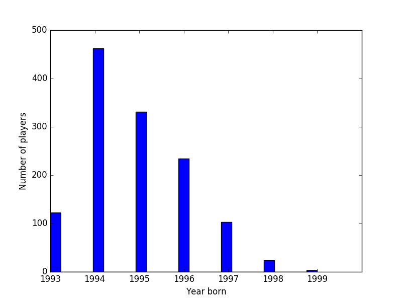
This is the end result. Pretty neat! Things learned here:
- Databases about something you remotely like are fun to explore.
- Visualizations are extremely useful in exploring data efficiently.
- There are 17 year old professional soccer players. I shouldn’t be suprised but I still am.